Stat-Ease Blog

Categories
Experimental Design in Chemistry: A Review of Pitfalls (Guest Post)
This blog post is from James Cawse, Consultant and Principal at Cawse and Effect, LLC. Jim uses his unique blend of chemical knowledge, statistical skills, industrial process experience, and quality commitment to find solutions for his client's difficult experimental and process problems. He received his Ph.D. in Organic Chemistry from Stanford University. On top of all that, he's a great guy! Visit his website (link above) to find out more about Jim, his background, and his company.
Introduction
Getting the best information from chemical experimentation using design of experiments (DOE) is a concept that has been around for decades, although it is still painfully underused in chemistry. In a recent article Leardi1 pointed this out with an excellent tutorial on basic DOE for chemistry. The classic DOE text Statistics for Experimenters2 also used many chemical illustrations of DOE methodology. In my consulting practice, however, I have encountered numerous situations where ’vanilla‘ DOE – whether from a book, software, or a Six Sigma course – struggles mightily because of the inherent complications of chemistry.The basic rationale for using a statistically based DOE in any science are straightforward. The DOE method provides:
- Points distributed in a rational fashion throughout “experimental space”.
- Noise reduction by averaging and application of efficient statistical tools.
- ‘Synergy’, typically the result of the interactions of two or more factors - easily determined in a DOE.
- An equation (model) that can then be used to predict further results and optimize the system.
DOE works so well in most scientific disciplines because Mother Nature is kind. In general:
- Most experiments can be performed with small numbers of ’well behaved‘ factors, typically simple numeric or qualitative at 2-3 levels
- Interactions typically involve only 2 factors. Three level and higher interactions are ignored.
- The experimental space is relatively smooth; there are no cliffs (e.g. phase changes).
Y = B0 + B1x1 + B2x2 + B12x1x2 + B11x12 +…
In contrast, chemistry offers unique challenges to the team of experimenter and statistician. Chemistry is a science replete with nonlinearities, complex interactions, and nonquantitative factors and responses. Chemical experiments require more forethought and better planning than most DOE’s. Chemistry-specific elements must be considered.
Mixtures
Above all, chemists make mixtures of ‘stuff’. These may be catalysts, drugs, personal care items, petrochemicals, or others. A beginner trying to apply DOE to a mixture system may think to start with a conventional cubic factorial design. It soon becomes clear, however, that there is an impossible situation when the (+1, +1, +1) corner requires 100% of A and B and C! The actual experimental space of a mixture is a triangular simplex. This can be rotated into the plane to show a simplex design, and it can easily be extended to high dimensions such as a tetrahedron.
It is rare that a real mixture experiment will actually use 100% of the components as points. A real experiment with be constrained by upper and lower bounds, or by proportionality requirements. The active ingredients may also be tiny amounts in a solvent. The response to a mixture may be a function of the amount used (fertilizers or insecticides, for example). And the conditions of the process which the mixture is used in may also be important, as in baking a cake – or optimizing a pharmaceutical reaction. All of these will require special designs.
Fortunately, all of these simple and complex mixture designs have been extensively studied and are covered by Cornell3, Anderson et al4, and Design-Expert® software.
Kinetics
The goal of a kinetics study is an equation which describes the progress of the reaction. The fundamental reality of chemical kinetics is
Rate = f(concentrations, temperature).
However, the form of the equation is highly dependent on the details of the reaction mechanism! The very simplest reaction has the first-order form
Rate = k*C1
which is easily treated by regression. The next most complex reaction has the form
Rate = k*C1*C2
in which the critical factors are multiplied – no longer the additive form of a typical linear model. The complexity continues to increase with multistep reactions.
Catalysis studies are chemical kinetics taken to the highest degree of complication! In industry, catalysts are often improved over years or decades. This process frequently results in increasingly complex catalyst formulations with components which interact in increasingly complex ways. A basic catalyst may have as many as five active co-catalysts. We now find multiple 2-factor interactions pointing to 3-factor interactions. As the catalyst is further refined, the Law of Diminishing Returns sets in. As you get closer to the theoretical limit – any improvement disappears in the noise!
Chemicals are not Numbers
As we look at the actual chemicals which may appear as factors in our experiments, we often find numbers appearing as part of their names. Often the only difference among these molecules is the length of the chain (C-12, 14, 16, 18) and it is tempting to incorporate this as numeric levels of the factor. Actually, this is a qualitative factor; calling it numeric invites serious error! The correct description, now available in Design-Expert, is ’Discrete Numeric’.
The real message, however, is that the experimenters must never take off their ’chemist hat‘ when putting on a ’statistics hat’!
Reference Materials:
- Leardi, R., "Experimental design in chemistry: A tutorial." Anal Chim Acta 2009, 652 (1-2), 161-72.
- Box, G. E. P.; Hunter, J. S.; Hunter, W. G., Statistics for Experimenters. 2nd ed.; Wiley-Interscience: Hoboken, NJ, 2005.
- Cornell, J. A., Experiments with Mixtures. 3rd ed.; John Wiley and Sons: New York, 2002.
- Anderson, M.J.; Whitcomb, P.J.; Bezener, M.A.; Formulation Simplified; Routledge: New York, 2018.
Greg’s DOE Adventure - Factorial Design, Part 1
[Disclaimer: I’m not a statistician. Nor do I want you to think that I am. I am a marketing guy (with a few years of biochemistry lab experience) learning the basics of statistics, design of experiments (DOE) in particular. This series of blog posts is meant to be a light-hearted chronicle of my travels in the land of DOE, not be a text book for statistics. So please, take it as it is meant to be taken. Thanks!]
So, I’ve gotten thru some of the basics (Greg's DOE Adventure: Important Statistical Concepts behind DOE and Greg’s DOE Adventure - Simple Comparisons). These are the ‘building blocks’ of design of experiments (DOE). However, I haven’t explored actual DOE. I start today with factorial design.
We can illustrate like this:
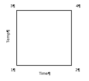
In this case, the horizontal line (x-axis) is time and vertical line (y-axis) is temperature. The area in the box formed is called the Experimental Space. Each corner of this box is labeled as follows:
1 – low time, low temperature (resulting in crunchy, matchstick-like pasta), which can be coded minus-minus (-,-)
2 – high time, low temperature (+,-)
3 – low time, high temperature (-,+)
4 – high time, high temperature (making a mushy mass of nasty) (+,+)
One takeaway at this point is that when a test is run at each point above, we have 2 results for each level of each factor (i.e. 2 tests at low time, 2 tests at high time). In factorial design, the estimates of the effects (that the factors have on the results) is based on the average of these two points; increasing the statistical power of the experiment.
Power is the chance that an effect will be found, when there is an effect to be found. In statistical speak, power is the probability that an experiment correctly rejects the null hypothesis when the alternate hypothesis is true.
If we look at the same experiment from the perspective of altering just one factor at a time (OFAT), things change a bit. In OFAT, we start at point #1 (low time, low temp) just like in the Factorial model we just outlined (illustrated below).
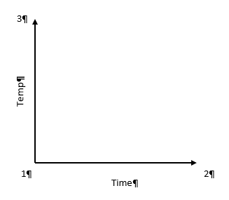
Here, we go from point #1 to #2 by lengthening the time in the water. Then we would go from #1 to #3 by changing the temperature. See how this limits the number of data points we have? To get the same power as the Factorial design, the experimenter will have to make 6 different tests (2 runs at each point) in order to get the same power in the experiment.
After seeing these results of Factorial Design vs OFAT, you may be wondering why OFAT is still used. First of all, OFAT is what we are taught from a young age in most science classes. It’s easy for us, as humans, to comprehend. When multiple factors are changed at the same time, we don’t process that information too well. The advantage these days is that we live in a computerized world. A computer running software like Design-Expert®, can break it all down by doing the math for us and helping us visualize the results.
Additionally, with the factorial design, because we have results from all 4 corners of the design space, we have a good idea what is happening in the upper right-hand area of the map. This allows us to look for interactions between factors.
That is my introduction to Factorial Design. I will be looking at more of the statistical end of this method in the next post or two. I’ll try to dive in a little deeper to get a better understanding of the method.
ASQ/ASA Fall Technical Conference Attendees - Sharpen those DOE Skills!
Expand your design of experiments (DOE) expertise at the 2019 Fall Technical Conference.
Martin Bezener will be teaching a pre-conference short course on Practical DOE and giving a session talk on binary data (abstracts are below). Shari Kraber will be hosting our exhibit booth and can discuss your DOE needs.
Short Course Abstract (Wed, Sep 25): Practical DOE: ‘Tricks of the Trade’
In this dynamic short-course, Stat-Ease consultant Martin Bezener reveals DOE tricks of the trade that make the most from statistical design and analysis of experiments. Come and learn many secrets for design of experiment (DOE) success, such as:
- How to build irregularly-shaped DOE spaces that cover your region of interest
- Using logistic regression to get the most from binomial data such as a pass/fail response
- Clever tweaks to numerical optimization
- Cool tools for augmenting a completed experiment to capture a peak beyond its reach
- Other valuable tips and tricks as time allows and interest expressed
Session 6A Abstract (Fri, Sep 27, 1:30pm): Practical Considerations in the Design of Experiments for Binary Data
Binary data is very common in experimental work. In some situations, a continuous response is not possible to measure. While the analysis of binary data is a well-developed field with an abundance of tools, design of experiments (DOE) for binary data has received little attention, especially in practical aspects that are most useful to experimenters. Most of the work in our experience has been too theoretical to put into practice. Many of the well-established designs that assume a continuous response don’t work well for binary data yet are often used for teaching and consulting purposes. In this talk, I will briefly motivate the problem with some real-life examples we’ve seen in our consulting work. I will then provide a review of the work that has been done up to this point. Then I will explain some outstanding open problems and propose some solutions. Some simulation results and a case study will conclude the talk.
Be sure to mark these as must attend events on your FTC schedule!
Hurry – Early Bird Registration ends Aug 25. Hotel block ends Aug 27. Final Registration ends September 13.
Links for more info:
How Can I Convince Colleagues Working on Formulations to Use Mixture Design Rather than Factorials or Response Surface Methods as They Would Do for Process Studies?
We recently published the July-August edition of The DOE FAQ Alert. One of the items in that publication was the question below, and it's too interesting not to share here as well.
Original question from a Research Scientist:
"Empowered by the Stat-Ease class on mixture DOE and the use of Design-Expert, I have put these tools to good use for the past couple of years. However, I am having to more and more defend why a mixture design is more appropriate than factorials or response surface methods when experimenting on formulations. Do you have any resources, blogs posts, or real-world data that would better articulate why trying to use a full factorial or central composite design on mixture components is not the most effective option?"
Answer from Stat-Ease Consultant Martin Bezener:
“First, I assume you are talking about factorials or response surface method (RSM) designs involving the proportions of the components. It makes no sense to use a factorial or RSM if you are dealing with amounts, since doubling the amount of everything should not affect the response, but it will in a factorial or response-surface model.
"There are some major issues with factorial designs. For one thing, the upper bounds of all the components need to sum to less than 1. For example, let’s say you experimented on three components with the following ranges:
A. X1: 10 - 20%
B. X2: 5 - 6%
C. X3: 10 - 90%
then the full-factorial design would lay out a run at all-maximum levels, which makes no sense as that gives a total of 116% (20+6+90). Oftentimes people get away with this because there is a filler component (like water) that takes the formulation to a fixed total of 100%, but this doesn't always happen.
"Also, a factorial design will only consider the extreme combinations (lows/highs) of the mixture. So, you'll get tons of vertices but no points in the interior of the space. This is a waste of resources, since a factorial design doesn't allow fitting anything beyond an interaction model.
"An RSM design can be ‘crammed’ into mixture space to allow curvature fits, but this is generally a very poor design choice. Using ratios of components provides a work-around, but that has its own problems.
"Whenever you try to make the problem fit the design (rather than the other way around), you lose valuable information. A very nice illustration of this was provided in the by Mark Anderson in his article on the “Peril of Parts & the Failure of Fillers as Excuses to Dodge Mixture Design” in the May 2013 Stat-Teaser.”
An addendum from Mark Anderson, Principal of Stat-Ease and author of The DOE FAQ Alert:
"The 'problems' Martin refers to for using ratios (tedious math!) are detailed in RSM Simplified Chapter 11: 'Applying RSM to Mixtures'. You can learn more about this book and the others in the Simplified series ('DOE' and 'Formulation') on our website."
Links for additional information:
- Back issues of The DOE FAQ Alert
- Signup to receive the bimonthly DOE FAQ Alert via email
- Learn more about mixture design by attending our computer-intensive workshop Mixture Design for Optimal Formulations
Greg’s DOE Adventure - Simple Comparisons
Disclaimer: I’m not a statistician. Nor do I want you to think that I am. I am a marketing guy (with a few years of biochemistry lab experience) learning the basics of statistics, design of experiments (DOE) in particular. This series of blog posts is meant to be a light-hearted chronicle of my travels in the land of DOE, not be a textbook for statistics. So please, take it as it is meant to be taken. Thanks!
As I learn about design of experiments, it’s natural to start with simple concepts; such as an experiment where one of the inputs is changed to see if the output changes. That seems simple enough.
For example, let’s say you know from historical data that if 100 children brush their teeth with a certain toothpaste for six months, 10 will have cavities. What happens when you change the toothpaste? Does the number with cavities go up, down, or stay the same? That is a simple comparative experiment.
“Well then,” I say, “if you change the toothpaste and 6 months later 9 children have cavities, then that’s an improvement.”
Not so fast, I’m told. I’ve already forgotten about that thing called variability that I defined in my last post. Great.
In that first example, where 10 kids got cavities. That result comes from that particular sample of 100 kids. A different sample of 100 kids may produce an outcome of 9, other times it’s 11. There is some variability in there. It’s not 10 every time.
[Note: You can and should remove as much variability as you can. Make sure the children brush their teeth twice a day. Make sure it’s for exactly 2 minutes each time. But there is still going to be some variation in the experiment. Some kids are just more prone to cavities than others.]
How do you know when your observed differences are due to the changes to the inputs, and not from the variation?
It’s called the F-Test.
I’ve seen it written as:
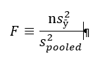
Where:
s = standard deviation
s2 = variance
n = sample size
y = response
ӯ (“y bar”) = average response
In essence, this is the amount of variance for individual observations in the new experiment (multiplied by the number of observations) divided by the total variation in the experiment.
Now that, by itself, does not mean much to me (see disclaimer above!). But I was told to think of it as the ratio of signal to noise. The top part of that equation is the amount of signal you are getting from the new condition; it’s the amount of change you are seeing from the established mean with the change you made (new toothpaste). The bottom part is the total variation you see in all your data. So, the way I’m interpreting this F-Test is (again, see disclaimer above): measuring the amount of change you see versus the amount of change that is naturally there.
If that ratio is equal to 1, more than likely there is no difference between the two. In our example, changing the toothpaste probably makes no difference in the number of cavities.
As the F-value goes up, then we start to see differences that can likely be credited to the new toothpaste. The higher the value of the F-test, the less likely it is that we are seeing that difference by chance and the more likely it is due to the change in the input (toothpaste).
Trivia
Question: Why is this thing called an F-Test?
Answer: It is named after Sir Ronald Fisher. He was a geneticist who developed this test while working on some agricultural experiments. “Gee Greg, what kind of experiments?”. He was looking at how different kinds of manure effected the growth of potatoes. Yup. How “Peculiar Poop Promotes Potato Plants”. At least that would have been my title for the research.